The Feature That Explained Everything (And Why It Wasn't in Your Dataset)

Rolling operational features, real-time data, and the 11-point AUC gap that changed how I think about prediction problems.

If you've ever built a predictive model on historical data and wondered why it performs worse than you'd expect on real-world inputs, this article is for you. My capstone project — predicting airline flight delays across 14 million flights — taught me something I didn't expect going in: the most important predictors aren't in most datasets.

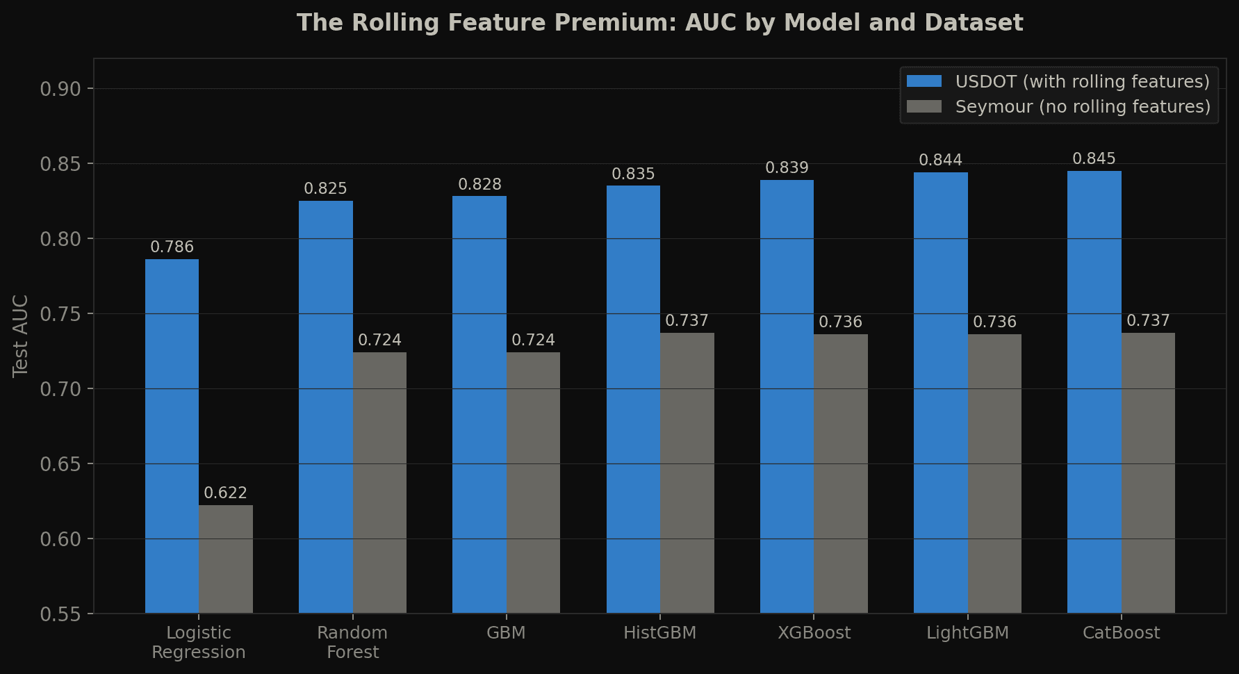
Every model — from logistic regression to CatBoost — performs roughly 10 points better on the USDOT dataset than on the Seymour dataset. Same model families, similar data volumes, completely different performance ceilings. The difference isn't model complexity. It's 60 features that only exist in one of them.

What rolling features actually are

Rolling features aggregate recent operational history across short time windows — 1 hour, 3 hours, 6 hours, up to 24 hours — grouped by airport, carrier, route, and individual aircraft tail number. They answer questions like: Is this airport currently running 40% delayed? Has this specific aircraft been delayed on its last three flights today?

These aren't sophisticated ML tricks. They're just lag features applied to a network of interconnected operations. The reason they work so well is that flight delays propagate. A delay in Atlanta at 7am doesn't stay in Atlanta — it cascades forward through every connection on that aircraft's day, radiates outward through passengers missing connections, and compounds as cascading late arrivals stack up at destination airports throughout the afternoon.

A static dataset — even a rich one with weather data — can't capture this. The Seymour dataset has 27 weather features and still peaked at 0.737 AUC. The USDOT dataset has one composite weather score and reached 0.845. That's the rolling feature premium in a single comparison.

What this means for any prediction problem

The lesson generalizes well beyond aviation. Anytime you're predicting outcomes in a network where recent history propagates forward — call center volume, server load, demand forecasting, customer churn — the most predictive features are almost always what's happening right now, not what happened historically. Static training datasets capture the historical distribution. They don't capture the current state of the system.

This has a practical implication: if you're building a model and wondering why it performs worse in production than on your test set, the first question worth asking is whether the test set captures the same temporal signal your training data does. If you trained on historical data and evaluated on held-out historical data, you may have implicitly evaluated in an easier regime than what you'll encounter live.

The operational tradeoff

Rolling features require live data. You can't precompute them at training time and ship them — they have to be recomputed continuously from a live feed, ideally every 15 minutes. That's a data engineering problem, not a modeling problem, and it's the difference between a model that works in a notebook and one that works in production.

For the capstone, the recommendation was explicit: deploy with rolling features only for flights departing within 12–24 hours. Outside that window, the model degrades toward the performance of a static historical model. The feature is only as good as the recency of its data.